By Tomas Rotta [tomasrotta.com]

This technical note examines a potential problem in computing prices of production (PP) from global input-output data using the eigenvalue approach, a central component of the Standard Interpretation of Marxian value theory.

I argue that, in empirical applications using global input-output data, the dominant eigenvalue of matrix A (the matrix of input-output coefficients) is highly sensitive to extreme outliers and to procedures intended to clean or winsorize the data.

This issue matters because, in the eigenvalue approach, the uniform profit rate is computed from the dominant eigenvalue of matrix M, which derives directly from matrix A. Consequently, both prices of production and the global uniform profit rate are highly sensitive to extreme observations and to the methods used to clean matrix A.

I refer to this phenomenon as “eigenvalue hacking,” because the estimated profit rate varies continuously with the outlier removal procedure. The term is analogous to “p-hacking” in econometrics, where p-values can be influenced by selective choices regarding the sample or the statistical specification.

Using global IO data from GLORIA, I will demonstrate how this issue can compromise the eigenvalue approach in the computation of PP and the global uniform profit rate. GLORIA comprises 1.2 terabytes of global input-output data, spanning 120 industries across 164 countries from 1990 to 2023. At the time of writing, its latest release is v060.

Assume all matrices have dimensions n x n, and all vectors are column vectors with dimensions n x 1. Row vectors (1 x n) are indicated by the transpose operator, superscript T. Then the following definitions apply.

Let Z be the squared matrix of input-output transactions, D the squared matrix of fixed capital depreciation, and x the gross output vector, all denominated in US dollars. To compute matrix A, we sum matrices Z and D and multiply their sum by the inverse of the diagonal matrix formed from the gross output vector (x):

Matrix A is therefore a squared matrix representing the input-output coefficients, adjusted for capital depreciation. This A matrix is central to the computation of PP in empirical work. However, as will become clear below, extreme outliers inside matrix A will jeopardize the reliability of the dominant eigenvalue computed from matrix M.

Prices of production (p) are hypothetical long-run prices that would attain under both profit-rate and wage-rate equalization. Let r denote the equalized profit rate, and w the equalized wage rate on a global scale. Then let L denote the employment vector adjusted both for skills (complex labor) and self-employment; and let l denote the direct labor coefficients (i.e., employment L per unit of gross output x, adjusted for skills and self-employment).

We evaluate matrix A and the vector $wl^{T}$ at prices of production, and add a profit margin on the constant and variable capital advanced. For a circulating capital model with no fixed capital (K), and wages advanced at the start of the production period, prices of production are given by:

In the Standard Interpretation, the uniform nominal wage (w) is endogenous because it is determined by evaluating the exogenously given workers’ consumption bundle (b) at production prices. Although the consumption bundle (b) is treated as exogenous, production prices (p) are endogenous. As a result, the nominal wage (w) is also endogenous:

Now we plug the nominal wage into the PP equation:

Note that $b{l}^{T}$ is an n x n matrix whose elements represent the quantity (or expenditure) of wage goods required to sustain the skill-adjusted and self-employment-adjusted labor associated with one unit of output in each industry.

The uniform profit rate (r) is a scalar. Thus, rearranging the equation:

Define lambda as:

We can now see that the PP model entails the simultaneous determination of prices (p) and the profit rate (r). As a result, the profit rate is not imposed from outside the system but emerges endogenously from the production-price model:

Define the augmented input matrix M:

Hence:

Or:

This is an eigenvalue problem: lambda is the eigenvalue associated with matrix $M=A+b{l}^{T}$; and the relative prices of production (p) are the left eigenvector of matrix M associated with the maximum eigenvalue $\lambda^{max}$. Note that the p vector multiplies matrix M from the left.

A common normalization for relative prices of production is that aggregate gross output evaluated at prices of production equals aggregate gross output at observed market prices. But this normalization is immaterial to the issue at hand.

Lambda max $(\lambda^{max})$ is the Perron–Frobenius root indicating the spectral radius $\rho(M)$ of matrix M. The uniform profit rate is given by solving $\lambda^{max} = 1/(1+r^{*})$ for $r^{*}$:

The Perron-Frobenius theorem states that if matrix M is non-negative and irreducible, its spectral radius $\rho(M)$ is a positive real eigenvalue and the associated left and right eigenvectors are strictly positive and unique up to multiplication by a positive scalar (i.e., the normalization condition). For the other eigenvalues to have strictly smaller modulus, we need the stronger condition that matrix M is also primitive.

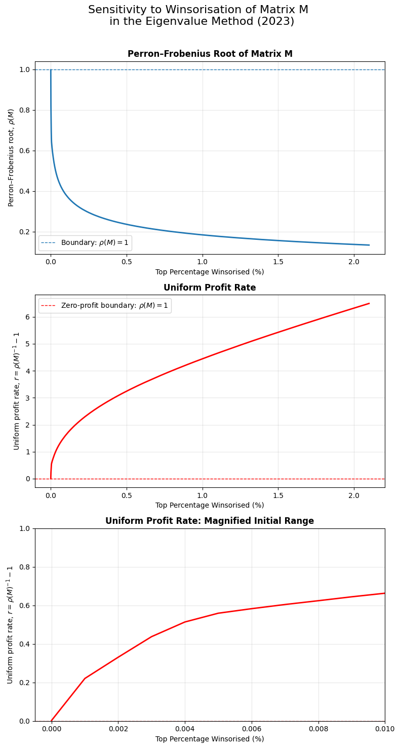
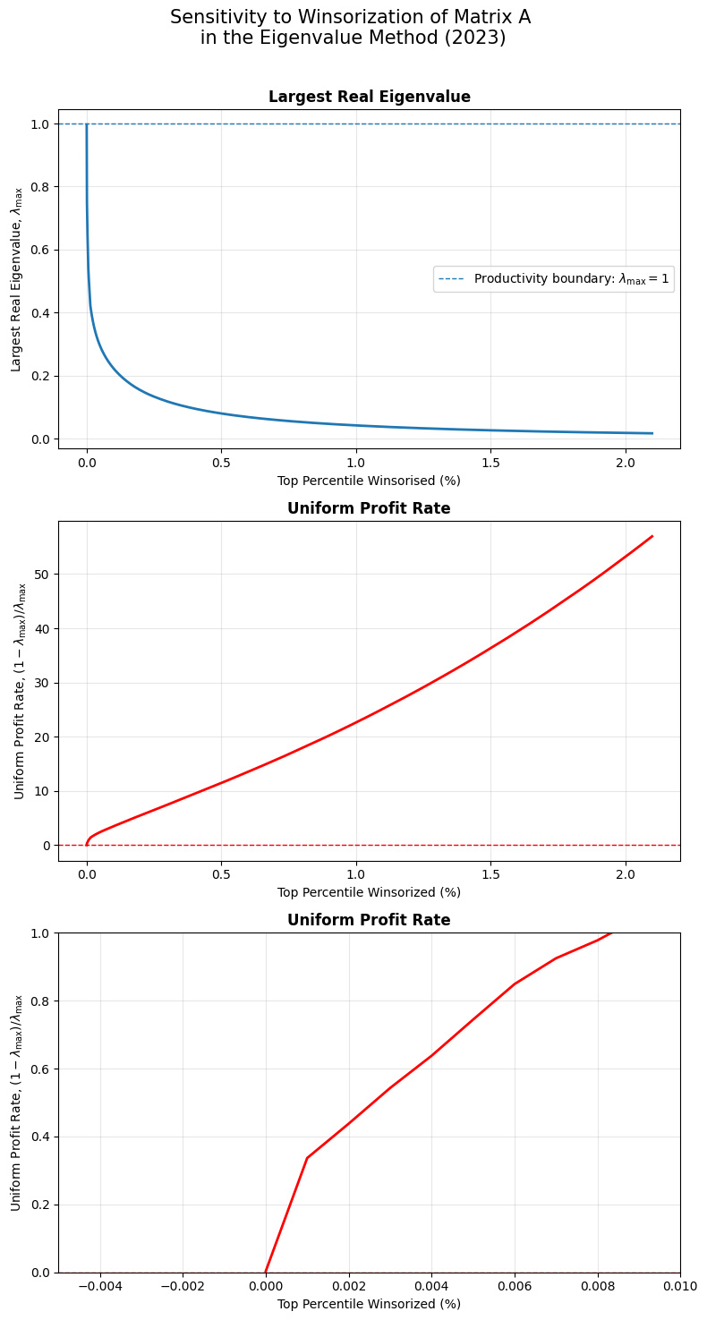
To illustrate the implications of eigenvalue hacking, I conducted a series of Python simulations using empirical IO data from GLORIA v060. The next figures show that even modest winsorization of matrix M can substantially alter the dominant eigenvalue and, consequently, the implied uniform profit rate.

Applying the eigenvalue approach to matrix M, computed from the 2023 GLORIA database, reveals that both the Perron–Frobenius root (i.e., the dominant eigenvalue) and the implied uniform profit rate are highly sensitive to extreme outliers. Even modest attempts to remove or cap these outliers in matrix M produce substantial changes in the dominant eigenvalue and, consequently, in the uniform profit rate. This sensitivity raises serious concerns about the reliability of the eigenvalue approach when applied to global input-output data.

When applied to national input-output data rather than global input-output data, the eigenvalue approach is likely to produce more reliable results because national statistical agencies, such as the U.S. Bureau of Economic Analysis (BEA), typically subject their input-output tables to extensive validation, balancing, and outlier treatment before public release. In contrast, extreme outliers are much more likely to arise in global input-output databases such as GLORIA, owing to the challenges of harmonizing and integrating data from many national sources. The main limitation of relying on national input-output data, however, is that they do not permit the computation of prices of production and a uniform profit rate at the global scale.

In the GLORIA database, matrix M has dimensions of 19,680 × 19,680, corresponding to 387,302,400 individual entries. Stored in double precision, a single annual matrix occupies approximately 3.3 GB of memory.

Winsorizing the matrix at the top 0.001% entails identifying the value that marks the upper 0.001% tail of the distribution and replacing all entries above this threshold with the threshold value itself. Entries below the threshold are left unchanged. For instance, if the threshold is 0.41, all values below 0.41 remain intact, while a value of 0.80 is capped at 0.41.

Notice how the uniform profit rate rises dramatically, from nearly zero to 0.60, even when only a handful of extreme outliers are capped:

.

.

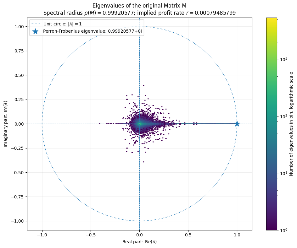
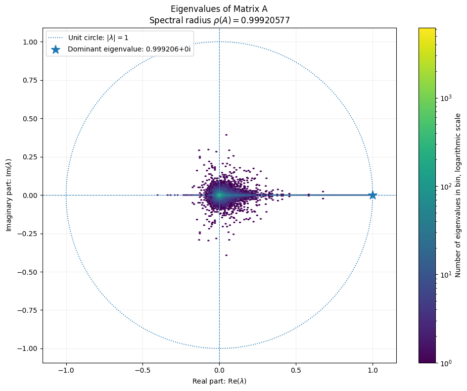
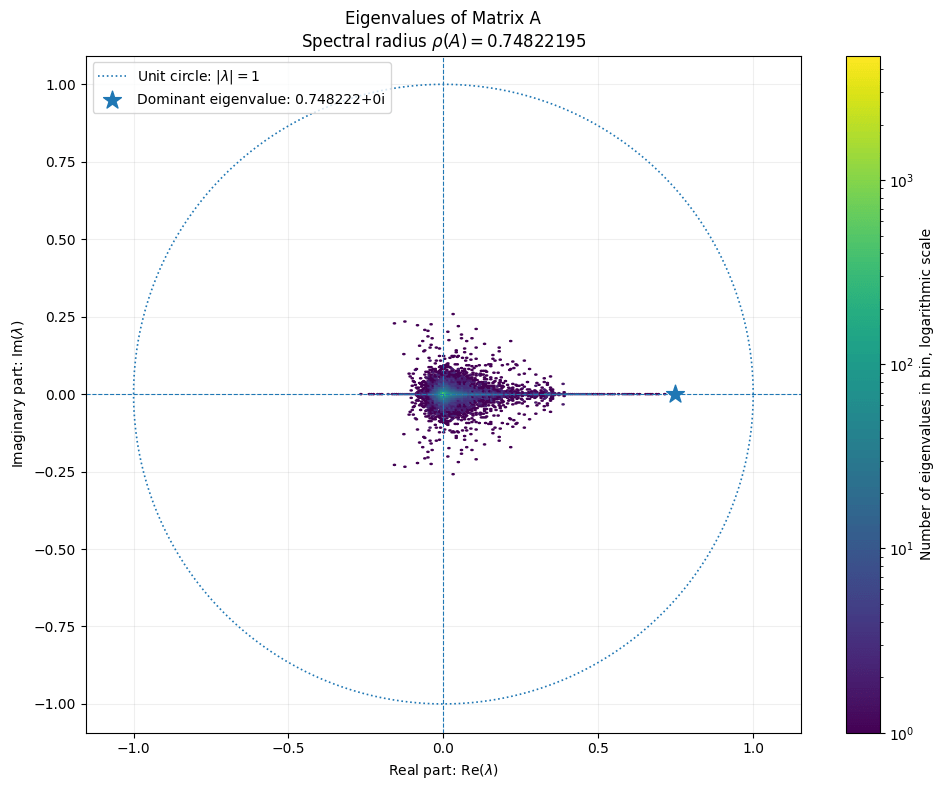
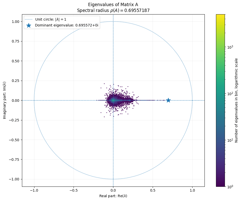
For a non-negative matrix M, the Perron-Frobenius root is real and nonnegative. The remaining eigenvalues, however, may be complex. Accordingly, I plot the eigenvalue spectrum in the complex plane, with the horizontal axis representing the real part and the vertical axis representing the imaginary part.

I include the unit circle as an economic reference because a positive uniform profit rate requires $\rho(M)<1$, in which case all eigenvalues of M lie inside the unit circle.

For the raw M matrix in 2023, prior to any winsorization, the dominant eigenvalue (i.e., the Perron-Frobenius root) is 0.999 and the implied profit rate is only 0.0008:

.

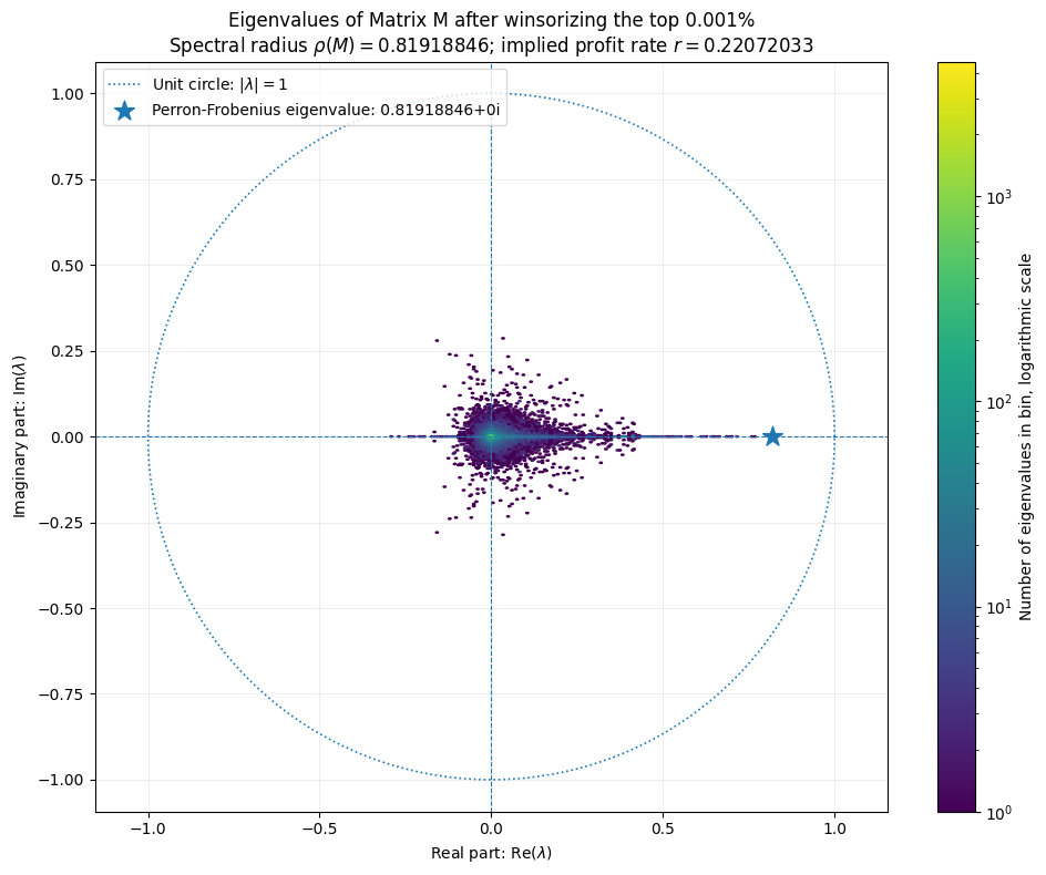
The following are the eigenvalues for the modified M matrix, after winsorizing the top 0.001% of outliers. The dominant eigenvalue drops to 0.82 and the implied profit rate rises to 0.22:

.

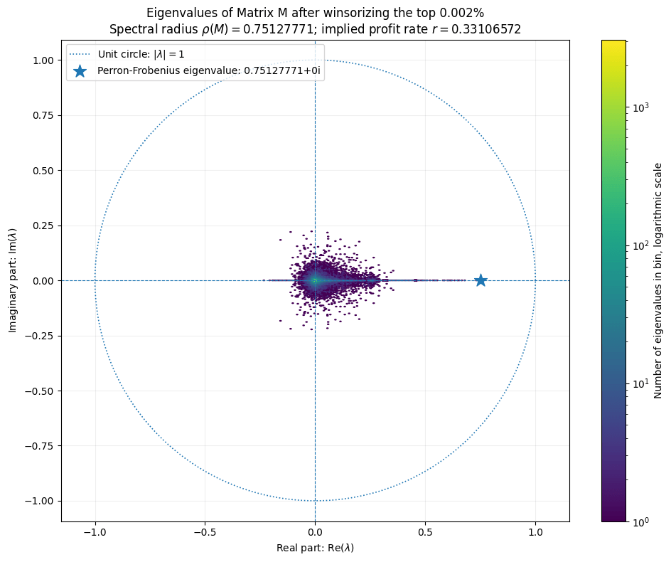
And the following are the eigenvalues for the modified M matrix after winsorizing the top 0.002% of outliers. The dominant eigenvalue drops even further to 0.75 and the implied profit rate rises even more to 0.33:

.

The central issue is that the eigenvalue approach provides no objective criterion for identifying which of the profit rates shown on the vertical axis should be regarded as the correct estimate. More importantly, the estimated profit rate can vary across nearly the entire range simply by changing the share of extreme outliers that are removed or capped in matrix M. This methodological indeterminacy is the essence of the “eigenvalue hacking” problem in the Standard Interpretation.

The source of the extreme-outlier problem lies in the input-output coefficients contained in matrix A, not in either the $bl^{T}$ matrix or matrix D.

The following figures show that the extreme outliers originate in matrix A:

.

.

These are the eigenvalues from the raw A matrix, with no winsorization:

.

These are the eigenvalues from the modified A matrix after winsorizing the top 0.001% of outliers:

.

Finally, these are the eigenvalues from the modified A matrix after winsorizing the top 0.002% of outliers:

.

If you have a solution to this problem using global input-output data, I would be very interested to hear it. Please share your thoughts in the comments below. I emphasize global because the same issue is much less likely to arise when working with national input-output data.

The challenge is not simply to compute prices of production from input-output data, since that can be done with national tables, but to do so robustly using a global input-output database, where the outlier problem emerges.

.

.

.

.

.